As I was saying last time, the 2022 physics Nobel Prize was awarded to John Clauser, Alain Aspect, and Anton Zeilinger for their contribution to quantum entanglement. This is associated with instantaneous “spooky action at a distance”, and is said to play an important role in quantum computing. It all started in 1935 with the EPR paper, where Einstein, Podolsky, and Rosen said quantum mechanics must be incomplete because it predicts a system in two different states at the same time. Bohr gave a rambling off-topic reply a few months later, talking about complementarity and the double slit experiment rather than the EPR paper, then claimed that spooky action at a distance could occur. Shortly thereafter Schrödinger came up with a paper where he talked about entanglement, followed by a paper where he used his cat to show how ridiculous the two-state situation was, followed by a paper saying he found spooky action at a distance to be repugnant. Schrödinger also compared the latter to Voodoo magic, where a savage “believes that he can harm his enemy by piercing the enemy’s image with a needle”.
 Voodoo doll by kloppstudio on DeviantArt
Then in 1952 Bohm came up with his two hidden variables papers, which were published back to back. Whilst he proposed hidden variables, he retained the spooky action at a distance. He also came up with Bohm’s variant in his 1951 textbook. It’s also known as the EPRB experiment, and was the subject of a paper in 1957 co-authored with Aharonov. It said there were complexities using spin ½ atoms, and talked instead about the photons resulting from electron-positron annihilation having “certain essential analogies to that of the spin measurement discussed in the previous section”. See journal page 1073. The paper also said “for the spin, these possibilities correspond to positive or negative spin in any chosen direction; and for the photon, they correspond to the two perpendicular directions in which the radiation oscillator can be excited”. In a nutshell, the paper said the only practical test was to use correlated photons and see if the polarizations were “perpendicular in every system of axes”.
On the Einstein Podolsky Rosen Paradox
After that came John Bell’s paper On the Problem of Hidden Variables in Quantum Mechanics. That’s where he said “In fact the Einstein-Podolsky-Rosen paradox is resolved in the way which Einstein would have liked least”. That was in 1964, before any experimental evidence, so I think it’s an unusual thing to say. As you can read on Scholarpedia, Bell wrote this paper before his famous 1964 paper On the Einstein Podolsky Rosen Paradox, but it didn’t get published until 1966 due to an “editorial accident”. Bell also wrote a lecture-notes paper in 1971 called Introduction to the Hidden-Variable Question, a paper called Bertlmann’s socks and the nature of reality in 1981, and a book in called Speakable And Unspeakable In Quantum Mechanics in 1987. However it’s his famous 1964 paper On the Einstein Podolsky Rosen Paradox that‘s of most interest here:
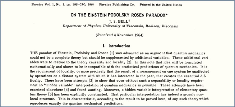
It’s only five pages long. In the introduction Bell said the idea of additional variables “will be formulated mathematically and shown to be incompatible with the statistical predictions of quantum mechanics”. He also referred to Bohm’s papers and said Bohm’s interpretation had a grossly non-local structure which was characteristic “of any such theory which reproduces exactly the quantum mechanical predictions”. Again I think it’s an unusual thing to say. Ditto for the quote in the Wikipedia Bell’s theorem article: “If a hidden-variable theory is local it will not agree with quantum mechanics, and if it agrees with quantum mechanics it will not be local”. Not only was there no evidence, but in section II Bell talked about singlet spin ½ particles and the use of Stern-Gerlach magnets to measure components of their spin, when he had no conceptual model of spin ½. You can’t describe a complex rotation with a +1 and a -1. In addition there’s an issue that Bohr would have understood: you can’t measure a particle without changing it in some way. For example, an electron goes round in circles in a uniform magnetic field because of Larmor precession. In similar vein the non-uniform Stern-Gerlach magnetic field alters the spin of a spin-up or spin-down silver atom. Bell had a degree in experimental physics, a degree in mathematical physics, and a physics PhD. But it’s as if he just didn’t care about the physics. He certainly didn’t care to make it clear that the Stern-Gerlach magnets are oriented at s different angles to conduct an EPR experiment.
Physics just doesn’t feature in his paper
Instead he launched into a mathematical “proof” that ended up with a declaration that “there must be a mechanism whereby the setting of one measuring device can influence the reading of another instrument, however remote”. I found that really unusual. It’s like saying you’ve come up with a mathematical proof for the existence of heaven and hell. It’s a non-sequitur. So is “moreover, the signal involved must propagate instantaneously”. How can anybody make such grandiose claims with no evidence? Especially when there were “realist” papers in the literature that ought to give pause for thought. See for example Charles Galton Darwin’s 1927 Nature paper on the electron as a vector wave, which talked about a spherical harmonic for the two directions of spin. It looks like Bell was promoting the Copenhagen Interpretation, so this sort of physics just doesn’t feature in his paper.
Bell’s inequality isn’t really Bell’s inequality
Rather surprisingly, nor does Bell’s inequality. Do a verbatim Google search on Bell’s inequality, and you will struggle to find the actual expression. That’s because Bell’s inequality isn’t really Bell’s inequality, and there’s considerable inconsistency. There’s a heavyweight Stanford article on Bell’s theorem, but the first inequality it gives is the 1969 CHSH inequality, in the form Sϱ(a,a′,b,b′) ≤ 2. It’s the same for the Wikipedia article on Bell’s theorem. The first inequality it gives is the CHSH inequality, in the form 〈A₀B₀〉 + 〈A₀B₁〉+ 〈A₁B₀〉 – 〈A₁B₁〉 ≤ 2. It does also give the expression:
|P(a, b) – P(a, c)| ≤ 1 + P(b, c)
This is Bell’s expression 15 flipped round. But the P here isn’t a probability, it’s a correlation, which isn’t quite the same thing. K Sugiyama gave some history in his article on the meaning of Bell’s inequality. He wrote Bell’s inequality in a different style as:
|C(A,W) − C(W,B)| ≦ 1 + C(A,B)
He also said “I think the meaning of the inequality is very difficult to understand”, and that Clauser and others improved things with the CHSH inequality, which he gave as:
|C(A,B) + C(A′,B) + C(A,B′) − C(A′,B′)| ≦ 2
But note that the Wikipedia article on the CHSH inequality says “The original 1969 derivation will not be given here since it is not easy to follow”. Sugiyama thought likewise, saying “I think the meaning of this inequality is also difficult to understand”. He also said Eugene Paul Wigner improved things further with the Wigner-d’Espagnat inequality of 1970, which he gave in this form:
P(A⁺;B⁺) ≦ P(A⁺;W⁺) + P(W⁺;B⁺)
This gave probabilities for a spin ½ EPR experiment with three measurement angles A B and W. For example P(A⁺;B⁺) is the probability that the left detector measures a +1 at angle A and the right detector measures a +1 at angle B. Sugiyama gives a link to a 1979 Sci-Am article on The Quantum Theory and Reality where Bernard d’Espagnat says this is the Bell inequality:
n[A⁺ B⁺] ≤ n[A⁺ C⁺] + n[B⁺ C⁺]
Sugiyama then says he thinks Bell’s inequality is more easily expressed as sets, and gave it in this form, albeit with a “not” on the last W term:
P(A∩B) ≦ P(A∩W) + P(W̅∩B)
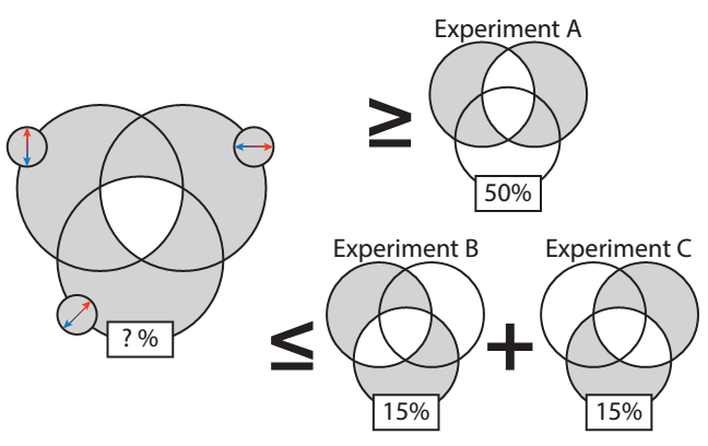
He also gave a Venn diagram to depict the above in graphical form. “Siggy”, a physics PhD, did the same in his article Bell’s Theorem explained. He described three experiments A B and C each measuring the spin of two entangled electrons at different angles, namely A: 0° and 90°, B: 0° and 45°, and C: 45° and 90°. He said quantum theory predicts a coincidence rate of (1+cos(x))/2, where x is the angle between measurements. This coincidence rate is the probability that both detectors will measure the same spin – Siggy said for simplicity he’s considering positive correlation. He then said “Under a hidden variable interpretation, each electron has a definite state even if it’s something you never measure”. And that every electron is either spin-up or spin-down, and either spin-left or spin-right, and either spin-up-right or spin-down-left. He then said this means every electron is in one of eight states, which you can summarize in a Venn diagram:
 Venn diagram from Siggy’s Bell’s Theorem explained
However the probabilities don’t make any sense. The probability that the electrons “are in the shaded region of the leftmost Venn diagram” must be greater than or equal to the 50% determined in experiment A. But “it must be no more than the sum of the shaded regions in the lower left diagrams, which we determined are 15% each, using experiments B and C”. Of course the probabilities don’t make any sense. That’s because the electron isn’t in one of eight states.
We can depict observations of a pair of entangled photons in a Venn diagram
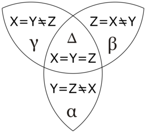
See the Wikiversity article on Bell’s theorem/Inequality for a similar argument with entangled photons and polarizing filters. It starts with a simple situation wherein the remote filter and a local filter are oriented in-line but with a 90° rotation from one another. Both are labelled X. The two entangled photons, which have orthogonal polarizations, either both pass through their respective filters or are both blocked. These two possibilities are assigned values X = +1 and X = -1. The article then adds two more local filters Y and Z which are 60° clockwise and anticlockwise of the first local filter. It then says the local photon must arrive at a measuring device with responses to all three polarization angles, and that “with three variables that can take on two possible values, we have eight possibilities”. So, if the remote photon passes through the remote filter then X = +1, if it’s blocked by the remote filter then X = -1, if the local photon passes through the 60° clockwise local filter then Y = +1, and so on. Since the two possible values are +1 and -1, at least two out of three X Y and Z values must equal each other, and we can depict our observations in a Venn diagram:
 CCASA Venn diagram by Guy Vandergrift, see Wikimedia Commons
Regions α β γ and Δ denote four mutually exclusive possibilities. If the remote photon passes through the remote filter X and its local partner passes through local filter Y but not Z, or the converse, that’s possibility γ, and so on. The probabilities sum to unity because only one possibility occurs per observation. Hence P(α) + P(β) + P(γ) + P(Δ) = 1. The article goes on to say there are two ways X=Y can occur, in regions γ and Δ, thus P(X=Y) = P(γ) + P(Δ). The same applies to Y=Z and Z=X, such that P(Y=Z) = P(α) + P(Δ), and P(Z=X) = P(β) + P(Δ). Combining all three gives us P(X=Y) + P(Y=Z) + P(Z=X) = P(α) + P(β) + P(γ) + 3 P(Δ) which is greater than 1. Hence “this leads to one version of Bell’s famous inequality”, given as:
P(X=Y) + P(Z=X) + P(Y=Z) ≥ 1
The article then says if the photon passed through filter X, the probability that it passes through filter Y is P(X=Y) = ¼, because cos²60° is 0.5 x 0.5, this being known as Malus’ law. Then it says P(X=Y) = P(Y=Z) = P(Z=X) = ¼. Hence:
P(X=Y) + P(Z=X) + P(Y=Z) = ¾
This contradicts the above version of Bell’s inequality. QED. Or, if you prefer: Shazam! I will talk about this some more next time. For now, this is said to be the EPR paradox.
Experimental Test of Local Hidden-Variable Theories
The experimental side of things is said to have started in 1969 with a paper describing a Proposed Experiment to Test Local Hidden-Variable Theories. The authors were John Clauser, Michael Horne, Abner Shimony, and Richard Holt (CHSH). It’s worth a read. It talks about Wu and Shaknov who in 1950 examined the polarization correlation of gamma rays emitted from positronium annihilation. It also talks about Carl Kocher and Eugene Commins who in 1966 examined the polarization correlation of photon pairs emitted from the radiative calcium cascade. They said “photons γ₁ and γ₂ are emitted successively, and their wavelengths are in the visible range (λ₁=5513 Å, λ₂=4227 Å)”. That’s interesting. As is this: “If a magnetic field is applied at the interaction region, an atom will precess during the time it spends in the intermediate state”. Kocher and Commins even mention Larmor precession. However, the CHSH guys said Kocher and Commins’ data didn’t suffice “because their polarizers were not highly efficient and were placed only in the relative orientations 0 and 90”. The CHSH paper then proposed an improved version of the Kocher and Commins experiment. The actual experiment was later described in the 1972 paper by Clauser and the late Stuart Freedman called Experimental Test of Local Hidden-Variable Theories.
The intermediate state lifetime of 5 nanoseconds
Oddly enough Clauser and Freedman are hardly mentioned in the Wikipedia Bell Test article. All it gives is a one-liner: “Stuart J Freedman and John Clauser carried out the first actual Bell test, using Freedman’s inequality, a variant on the CH74 inequality[11]”. Reference 11, which is supposed to be the Clauser and Freedman paper, links to Freedman’s 1972 PhD thesis, which was also called Experimental Test of Local Hidden-Variable Theories. Clauser and Freeman’s paper of the same name is just over three pages long. It says they measured the correlation in linear polarization of two photons γ₁ and γ₂ emitted in a J=0➝J=1➝J=0 atomic cascade. “The decaying atoms were viewed by two symmetrically placed optical systems, each consisting of two lenses, a wavelength filter, a rotatable and removable polarizer, and a single-photon detector”. There’s also a coincidence detector. They say the intermediate state lifetime of 5 nanoseconds permitted a narrow coincidence window of 8.1 nanoseconds. That’s interesting. They also said the typical coincidence rate with polarizers removed ranged from 0.3 to 0.1 counts per second. Freedman’s inequality is given as expression (3) at the bottom of the second page:
δ = | R(22½ °) / R₀ – R(67½ °) / R₀ | – ¼ ≤ 0
R is the coincidence rate for two-photon detection with both polarizing filters in place, and R₀ is the coincidence rate for two-photon detection with no polarizing filters. The paper includes this punchline: “This Letter reports the results of an experiment which are sufficiently precise to rule out local hidden-variable theories with high statistical accuracy”. Here’s the graph showing their results. Note that it resembles a cosine plot:
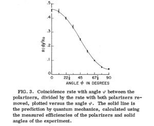 Image from Experimental Test of Local Hidden-Variable Theories by Clauser and Freedman
The moot point is that R(22½°)/R₀ is about 0.4, R(67½°)/R₀ is about 0.1, so δ = 0.4 – 0.1 – 0.25 = 0.05. There’s a SciTechDaily article about the experiment that’s well worth reading. See First Experimental Proof That Quantum Entanglement Is Real. Note that “Clauser’s work earned him the 2010 Wolf Prize in physics. He shared it with Alain Aspect… and Anton Zeilinger…’for an increasingly sophisticated series of tests of Bell’s inequalities, or extensions thereof, using entangled quantum states’”. Clauser gives an interview saying “My faculty at Columbia told me that testing quantum physics was going to destroy my career”. He also said “Richard Feynman was highly offended by my impertinent effort and told me that it was tantamount to professing a disbelief in quantum physics. He arrogantly insisted that quantum mechanics is obviously correct and needs no further testing!” In addition he said “I found Einstein’s ideas to be very clear. I found Bohr’s rather muddy and difficult to understand”. Clauser also said he was very sad to see that his own experiment had proven Einstein wrong. He also talked about the CH74 inequality which was contained in the 1974 paper Experimental consequences of objective local theories. See John Clauser’s website for more, including his 1976 paper Experimental investigation of a polarization correlation anomaly.
The Aspect Experiment
Alain Aspect is generally said to have conducted improved Bell test experiments. Funnily enough the Wikipedia article on the Aspect experiment says “Aspect’s experiment was the first quantum mechanics experiment to demonstrate the violation of Bell’s inequalities”. It doesn’t even mention Clauser and Freedman’s experiment. See the 1981 paper Experimental Tests of Realistic Local Theories via Bell’s Theorem by Alain Aspect, Philippe Grangier, and Gérard Roger. This refers to Clauser and Freedman plenty of times, and describes an experiment that’s essentially the same as Clauser and Freedman’s. It still features a calcium cascade, but the atomic beam of calcium is excited by two lasers producing far more photon emissions. The photons are “correlated in polarization”. (In A Brief Description of Aspect’s Experiment, Frank Rioux says they’re emitted in opposite directions with the same circular polarization according to the observers in their path). Aspect et al also moved each polarizer up to 6.5 metres from the source. A second paper, dating from 1982, was called Experimental Realization of Einstein-Podolsky-Rosen-Bohm Gedankenexperiment: A New Violation of Bell’s Inequalities. This described an experiment which replaced ordinary polarizers with two-channel polarizers “separating two orthogonal linear polarizations”. Each polarizer is made of two prisms, and transmits parallel polarized light whilst reflecting perpendicular polarized light, into two different photon detectors:
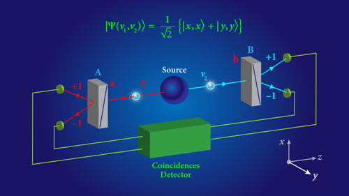 Image credit APS/Alan Stonebraker, see Closing the Door on Einstein and Bohr’s Quantum Debate
Later that year came Experimental Test of Bell’s Inequalities Using Time-Varying Analyzers with Jean Dalibard instead of Philippe Grangier. This is where they used ultrasound in water to rapidly deflect the photons to another polarizer oriented at a different angle, thereby changing the settings during the flight of the particles as suggested by Bell. All the papers feature a cosine-like curve. Note that the Wikipedia Aspect experiment article says this: “Bell’s inequalities establish a theoretical curve of the number of correlations (++ or −−) between the two detectors in relation to the relative angle of the detectors (α – β). The shape of the curve is characteristic of the violation of Bell’s inequalities”. The article gives the expression below:
P++(α,β) = P–(α,β) = ½ cos²(α – β)
In a nutshell, this is saying the probability of both photons going through filters 90° apart is zero, because cos 90° is zero. If however the polarizers are 0° apart the probability is 1, whilst at angles between the two the probability follows a cosine-like curve. See the 1999 Nature paper Bell’s inequality test: more ideal than ever for some background, along with Aspect’s 2007 Nature review paper To be or not to be local. In addition there’s the 2015 APS article Closing the Door on Einstein and Bohr’s Quantum Debate where Aspect gives a historical round-up of events.
Violation of Bell’s inequality under strict Einstein locality conditions
A further Bell test was performed in Innsbruck in 1998 by Gregor Weihs, Thomas Jennewein, Christoph Simon, Harald Weinfurter, and Anton Zeilinger. Their paper was Violation of Bell’s inequality under strict Einstein locality conditions. It starts by talking about “The stronger-than-classical correlations between entangled quantum systems, as first discovered by Einstein, Podolsky, and Rosen”. Somehow I don’t think that was the point Einstein, Podolsky, and Rosen were making. The paper also talks about “Bell’s discovery that EPR’s implication to explain the correlations using hidden parameters would contradict the predictions of quantum physics”. That’s one of those mathematical “discoveries” that is usually bereft of evidence. The paper goes on to talk about loopholes, in particular the communication loophole, saying Aspect et al had left the latter open. Aspect et all didn’t rotate the analyzers during the flight of the particles, they only used periodical sinusoidal switching, thus “communication slower than the speed of light, or even at the speed of light, could in principle explain the results obtained”. To close the loophole the Innsbruck team used detectors that were 400m apart, and performed their measurements in less than 1.3 μs to ensure they had a spacelike separation. They used type-II parametric down-conversion to generate the photon pairs with opposite polarizations, with a rapid switching of the detector orientation via an electro-optic modulator and random number generator. Near the end of the paper they said this: “Quantum theory predicts a sinusoidal dependence for the coincidence rate C++(α, β) ∝ sin²(β – α) on the difference angle of the analyzer directions in Alice’s and Bob’s experiments”. They gave this image which shows the same cosine-like curve as all the other papers:
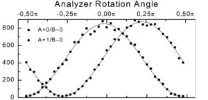 Part of figure 3 from Violation of Bell’s Inequality under Strict Einstein Locality Conditions by Zeilinger et al
They also said “Thus, for various combinations of analyzer directions α, β, α’, β these functions violate Bell’s inequality”. At the very end they said a shift of our classical philosophical positions seems necessary. They finished up with this: “Whether or not this will finally answer the eternal question: ‘Is the moon there, when nobody looks?’ [18], is certainly up to the reader’s personal judgment”. Trust me dear reader, the Moon is there, whether you look at it or not. Oh what an entangled web we weave. Not just because a photon travels 1.5m in 5 nanoseconds. Because of Malus’s law too. And because that heavyweight Stanford article I mentioned says this: “In Bell’s toy model, correlations fall off linearly with the angle between the device axes”.
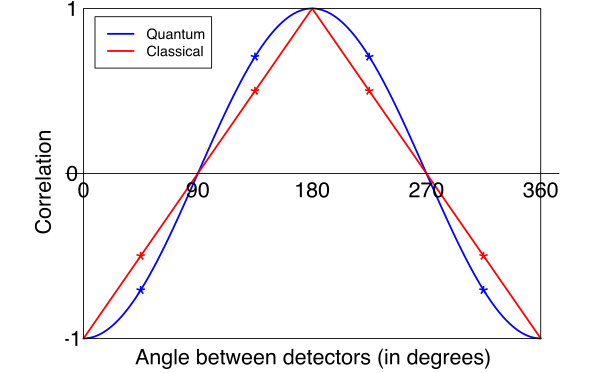 CCASA image by Richard Gill, see
Hi John, thank you for the deep dive into this topic, I was hoping you would cover this since there is so much misunderstanding regarding this topic and as usual the majority draws the wrong conclusions…
You went way more elaborate I could hope for, but in a sense that also muddles the waters a bit, so I would like to summarize how I see it: all the results that were done were nothing but experiments that showed the behavior of polarizers (following Malus Law). that is why there is no violation at angles 90, 0 and 45… To me it is bizarre that nobody in the regular science media sees this.
I think part of all the misunderstanding is that they keep holding on to the supposedly particle aspect: it goes through the polarizer or not (in reality since photons and electrons are waves/disturbances in eather you get as result intensity changes (described by Malus law)). Also thanks for pointing out the mess with the actual equation, intuitively I feel there is a lot of misinterpretation and a lot of assumptions, a mathematical exercise which has no grounds in reality.
One last thing is the single photon detector, I heard this is a very tricky thing to do, is this something we really can do with accuracy? I can imagine that if you put a polarizer in the path you get a more statistical/probabilistic outcome, which then also explains the results…
So for me there is nothing mysterious or non-local going on (or disproving hidden variables), the entangled particles (I don’t like to call them that but for the sake of argument) leave the source with all properties defined/set. The properties are not magically appearing afterwards by collapsing the wavefunction, what is happening is merely a result of how they measure it, and in this case they don’t seem to understand the implications of using polarizers…
Good stuff, keep it coming!
Thanks Raf. I find all the assertions about quantum entanglement utterly astonishing myself. I had to bite my tongue whilst writing about the history and the various papers and articles as per the above. At one point whilst writing this article I referred to https://physicsdetective.com/what-is-a-photon/ and the polarizers here: http://hyperphysics.phy-astr.gsu.edu/hbase/phyopt/polcross.html#c1. However I ended up taking it out because the article ended up being too long. Malus’s law means you are going to get a cosine-like curve. And yet that is used as proof positive of some magical mysterious spooky action at a distance. Because Bell’s inequality translates into some straight line chart? Not only that, but Clauser’s photons were separated by 5 ns. That’s 1.5m. They were never even entangled in the first place. Ditto for Aspect. Which means quantum entanglement is a castle in the air, built of layer upon layer of crap, held up by hype and hot air. FFS.
.
I may delete this comment tomorrow.
Maybe you could add a summary at the end to paraphrase the salient point of this blog post. As it is I found it somewhat hard to follow.
Sorry Leon. I’ll see what I can do.
Please don’t delete Sir ! Let it stand !
” quantum entanglement is a castle in the air, built up of layer of layer of crap, held up by hype and hot air. ” Now my Granny completely, unequivocally understands that quantum entanglement is BOGUS . And so do more and more other scientists and writers as of late; especially concerning the whole computing qubits quagmire scam……….
Just you wait until the next article Greg.
Hey,
Have you read Thomas Kuhn’s “The Structure of Scientific Revolutions”?
Eric: yes. I’ve just dug my copy out of my bookshelf. It’s a third edition, printed in 1996. I have a whole host of physics books. It might be fun to reread some of them in the light of what I now know. But there again, it might not be.
I tweaked the title to add the word history, so that the next article would be free-standing. I was going to call it Quantum Entanglement III, but changed my mind when I realised the extent of the issue. I also changed the last picture in this article.
I firmly believe that entanglement is just a concept to explain correlations between measurement results and nothing else. All of the magic can be fully explained by Malus’ law which describes the intensity of light based on the relative angle of polarizer settings. I’ve looked very closely at just about all aspects of Bell’s theorem/inequality, and cannot identify a single part of his analysis where he carefully proved any of the broad sweeping conclusions about locality, realism, and implications of non-locality. The only way to accurately describe how this type of physical system works is to develop a working model to highlight the nature of the underlying variables.
Good stuff Brian. You might like to click on NEXT to view the next article. Or view this article: There is no quantum entanglement.
Apologies if the Captcha is being over zealous. I had to click on about four images. Grrrr.
“Parts is Parts” is the new quantum entanglement: The biggest machine in science: inside the fight to build the next giant particle collider …
Thank you Dredd. I’m afraid collider physics is on a par with looking at firework explosions and thinking they will teach you how to make gunpowder.
I just sent you emails with my two cents worth of A.I. inspired word & math salad.
Titled : What I did on my Permanent Summer Vacation. Vols.1 & 2.
I consider this a positive, fun exercise in social science/ human psychology; as much as something posing as possible science.
Noted, Greg. Only it isn’t really the Duffield model. The photon stuff comes from What is a photon? and other papers. The electron stuff comes from Williamson and van der Mark and other papers, and so on. I’m not a “my theory” guy. I’m just a no shit Sherlock guy with a historian sideline.
Yes, and that is exactly why it needs your editorial prowess. Please forward all and any more corrections via email so you don’t waste Blog space. I strive for 💯 accuracy, even though I am a rookie layman wannabe myself . LOL 😆
More critique of Alain Aspect experiment just arrived:
https://www.youtube.com/watch?v=tI_ZqrdUigI&t=1638s
In general, the channel is offering great videos on hot topic in new physics (No Big Bang, dark energy wrong etc).
https://www.youtube.com/@SeethePattern
Thanks Dmitriy. I’ll have a look.
Basically, nobody liked non-locality since 100 years ago. Everyone tried to prove it wasn’t necessary. Eventually, it was shown what experimental results would prove non-locality was real (Bell’s theorems). Experiments followed, all showing non-locality to be present.
.
In this video, the last part where the spin rotates to align to the field, that’s what happens to the first particle. However, the second particle also rotates to align with the field before it’s measured. Measuring the first particle makes the second one rotate to align as well (that’s the spooky action). For example, with light, the first polarizer that makes the first photon align with the polarization axis, but it also immediately makes the second entangled photon align as well, and then the second photon will go through a polarizer at the same orientation with 100% chance.
.
If this interpretation (hidden variable) in the video was true, somebody would publish or post online the hidden variable that somehow has alluded everyone else for 100 years. You could even make a simple computer program to produce results equivalent to measured results. Nobody has managed to do either of these, and in fact, it has been shown in several different ways that no local hidden variable you can imagine can produce the results we see.
.
I don’t see the issue with non-locality, never have. So far it seems like the lower limit on the speed of the spooky action is 10,000 c, they keep increasing the lower limit as they expand the distance between detectors. I wonder if there is a max speed non-locality moves at, or if it’s really instant.
Doug, this is quackery, and sorry to say but you sound like a quack. By your logic all we have to do is place detectors on different galaxies and then we can “PROVE” the speed of spooky action at a distance is 100,000,000,000 c! Then if we extend it further we can eventually “PROVE” that spooky action at a distance can travel the entire length of the known universe instantaneously! Wow! How Great! How about we make up the spooky action at a distance particle? It is massless and can carry no information, but it collapses wave functions perfectly AND only the wave function for 1 other particle in the universe! How amazingly selective! We will call it the Quack Charm particle.
.
There are no photons that are “entangled”. Entanglement itself is a myth, its fantasy deduced up by some equations on paper, and extrapolated to ridiculous extremes…
Andy: your ignorance is entertaining as always, the goose crying about quacks! Your choice of remaining ignorant though is baffling. Especially now that you could just ask chatGPT!